4. AdEx: the Adaptive Exponential Integrate-and-Fire model
Book chapters
The Adaptive Exponential Integrate-and-Fire model is introduced in Chapter 6 Section 1
Python classes
Use function AdEx.simulate_AdEx_neuron() to run the model for different input currents and different parameters. Get started by running the following script:
% matplotlib inline
import brian2 as b2
from neurodynex.adex_model import AdEx
from neurodynex.tools import plot_tools, input_factory

current = input_factory.get_step_current(10, 250, 1. * b2.ms, 65.0 * b2.pA)
state_monitor, spike_monitor = AdEx.simulate_AdEx_neuron(I_stim=current, simulation_time=400 * b2.ms)
plot_tools.plot_voltage_and_current_traces(state_monitor, current)
print("nr of spikes: {}".format(spike_monitor.count[0]))
# AdEx.plot_adex_state(state_monitor)
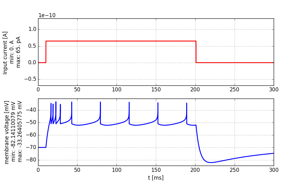
Step current injection into an AdEx neuron.
4.1. Exercise: Adaptation and firing patterns
We have implemented an Exponential Integrate-and-Fire model with a single adaptation current w:
4.1.1. Question: Firing pattern
- When you simulate the model with the default parameters, it produces the voltage trace shown above. Describe that firing pattern. Use the terminology of Fig. 6.1 in Chapter 6 Section 1
- Call the function
AdEx.simulate_AdEx_neuron()with different parameters and try to create adapting, bursting and irregular firing patterns. Table 6.1 in Chapter 6 Section 1 provides a starting point for your explorations. - In order to better understand the dynamics, it is useful to observe the joint evolution of
uandwin a phase diagram. Use the functionAdEx.plot_adex_state()to get more insights. Fig. 6.3 in Chapter 6 Section 2 shows a few trajectories in the phase diagram.
Note
If you want to set a parameter to 0, Brian still expects a unit. Therefore use a=0*b2.nS instead of a=0.
If you do not specify any parameter, the following default values are used:
MEMBRANE_TIME_SCALE_tau_m = 5 * b2.ms
MEMBRANE_RESISTANCE_R = 500*b2.Mohm
V_REST = -70.0 * b2.mV
V_RESET = -51.0 * b2.mV
RHEOBASE_THRESHOLD_v_rh = -50.0 * b2.mV
SHARPNESS_delta_T = 2.0 * b2.mV
ADAPTATION_VOLTAGE_COUPLING_a = 0.5 * b2.nS
ADAPTATION_TIME_CONSTANT_tau_w = 100.0 * b2.ms
SPIKE_TRIGGERED_ADAPTATION_INCREMENT_b = 7.0 * b2.pA
4.2. Exercise: phase plane and nullclines
First, try to get some intuition on shape of nullclines by plotting or simply sketching them on a piece of paper and answering the following questions.
- Plot or sketch the u- and w- nullclines of the AdEx model (
I(t) = 0) - How do the nullclines change with respect to
a? - How do the nullclines change if a constant current
I(t) = cis applied? - What is the interpretation of parameter
b? - How do flow arrows change as
tau_wgets bigger?
4.2.1. Question:
Can you predict what would be the firing pattern if a is small (in the order of 0.01 nS) ? To do so, consider the following 2 conditions:
- A large jump
band a large time scaletau_w. - A small jump
band a small time scaletau_w.
Try to simulate the above conditions, to see if your predictions were true.
4.2.2. Question:
To learn more about the variety of patterns the relatively simple neuron model can reproduce, have a look the following publication: Naud, R., Marcille, N., Clopath, C., Gerstner, W. (2008). Firing patterns in the adaptive exponential integrate-and-fire model. Biological cybernetics, 99(4-5), 335-347.